This example is taken from the ProBound web server, and corresponds to Figure 6 in the original Nature Biotech publication.

This example produces a model of the sequence-specificity of the tyrosine kinase c-Src by training on data from a Kinase-seq experiment, in which a bacterial display peptide library is exposed to c-Src and anti-phosphotyrosine pulldowns are performed at varying timepoints, which are modeled jointly.

import torch
import scipy.stats
import matplotlib.pyplot as plt

import pyprobound
import pyprobound.plotting
import pyprobound.fitting

Data specification

alphabet = pyprobound.alphabets.Protein()

url = "http://pbdemo.x3dna.org/files/example_data/Kinase/"

dataframes = [
    pyprobound.get_dataframe(f"{url}countTable.0.200205_Src-Kinase_5m.tsv.gz"),
    pyprobound.get_dataframe(
        f"{url}countTable.1.200205_Src-Kinase_20m.tsv.gz"
    ),
    pyprobound.get_dataframe(
        f"{url}countTable.2.200205_Src-Kinase_60m.tsv.gz"
    ),
]

count_tables = [
    pyprobound.CountTable(
        dataframe,
        alphabet,
        left_flank="TAGTSVAGQSGQ",
        right_flank="GGQSGQSGDYNK",
        left_flank_length=3,
        right_flank_length=3,
    )
    for dataframe in dataframes
]

Model specification

PSAMs

nonspecific = pyprobound.layers.NonSpecific(alphabet=alphabet, name="NS")
psam = pyprobound.layers.PSAM(
    kernel_size=7,
    alphabet=alphabet,
    pairwise_distance=6,
    seed=["***Y***"],
    seed_scale=45,
    symmetry=list(range(1, 8)),
    frozen_parameters=pyprobound.layers.PSAM.frozen_positions(
        [4], symmetry=list(range(1, 8)), out_channels=1, in_channels=20
    ),
    name="Src",
)

Modes

modes = [
    pyprobound.Mode.from_nonspecific(nonspecific, count_tables[0]),
    pyprobound.Mode.from_psam(psam, count_tables[0]),
]

Rounds

round_0_5m = pyprobound.rounds.InitialRound()
round_1_5m = pyprobound.rounds.ExponentialRound.from_binding(
    modes, round_0_5m, delta=-15, train_delta=False, target_concentration=0.25
)

round_0_20m = pyprobound.rounds.InitialRound()
round_1_20m = pyprobound.rounds.ExponentialRound.from_round(
    round_1_5m, round_0_20m, target_concentration=1.0
)

round_0_60m = pyprobound.rounds.InitialRound()
round_1_60m = pyprobound.rounds.ExponentialRound.from_round(
    round_1_5m, round_0_60m, target_concentration=3.0
)

Experiments

experiments = [
    pyprobound.Experiment(
        [round_0_5m, round_1_5m],
        name="Src-5m",
        counts_per_round=count_tables[0].counts_per_round,
    ),
    pyprobound.Experiment(
        [round_0_20m, round_1_20m],
        name="Src-20m",
        counts_per_round=count_tables[1].counts_per_round,
    ),
    pyprobound.Experiment(
        [round_0_60m, round_1_60m],
        name="Src-60m",
        counts_per_round=count_tables[2].counts_per_round,
    ),
]

Model

model = pyprobound.MultiExperimentLoss(experiments, pseudocount=50)

Fitting

optimizer = pyprobound.Optimizer(
    model,
    count_tables,
    greedy_threshold=2e-4,
    device="cpu",
    checkpoint="Src.pt",
    output="Src.txt",
)

optimizer.train_sequential()

tensor(2.3807)

optimizer.reload()

{'time': 'Tue Apr 23 19:42:08 2024',
 'version': '1.3.1',
 'flank_lengths': ((3, 3), (3, 3), (3, 3))}

Loss

with torch.inference_mode():
    loss, reg = model(count_tables)
    print(loss, reg, loss + reg)

tensor(0.5172) tensor(1.8635) tensor(2.3807)

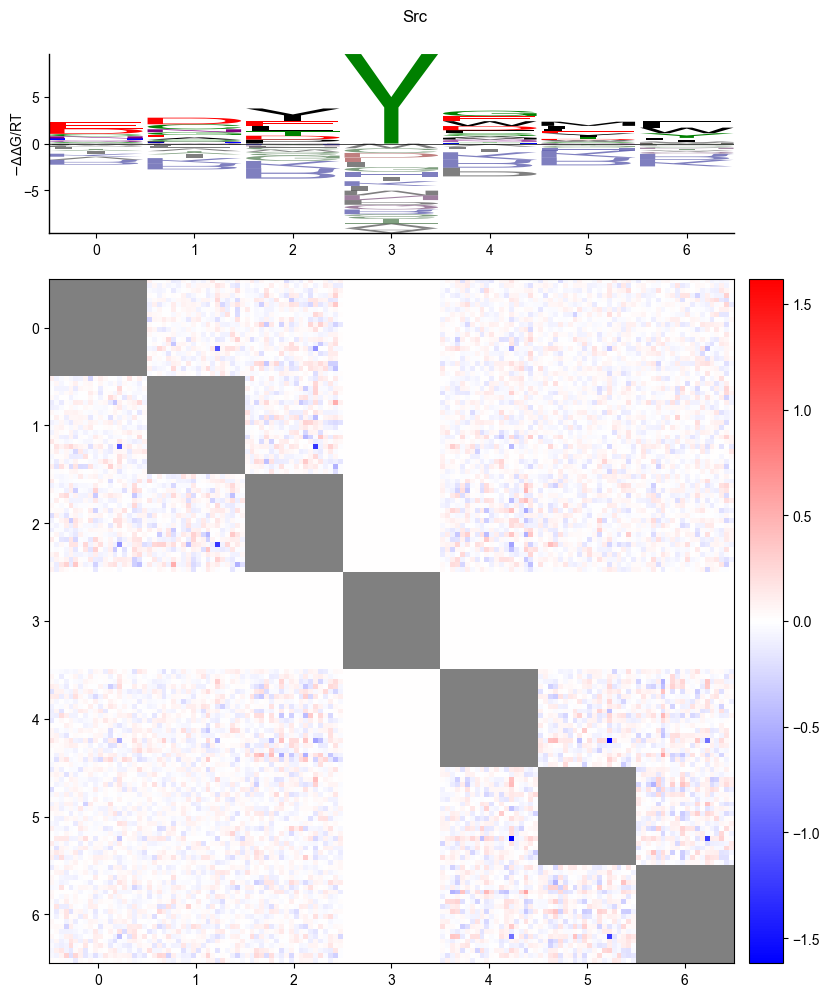
Logo

pyprobound.plotting.logo(psam)

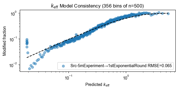
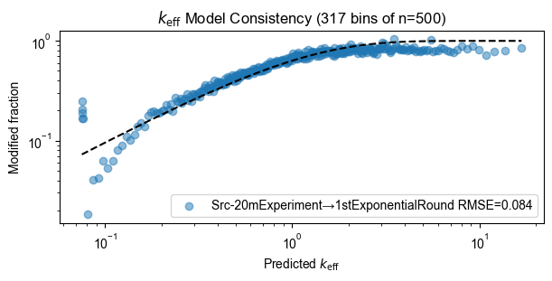
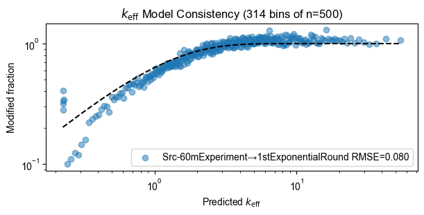
Model consistency

for experiment, count_table in zip(experiments, count_tables):
    pyprobound.plotting.keff_consistency(experiment, count_table)

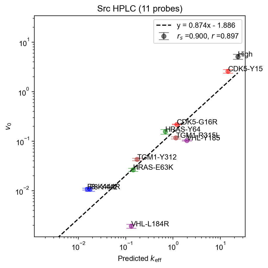
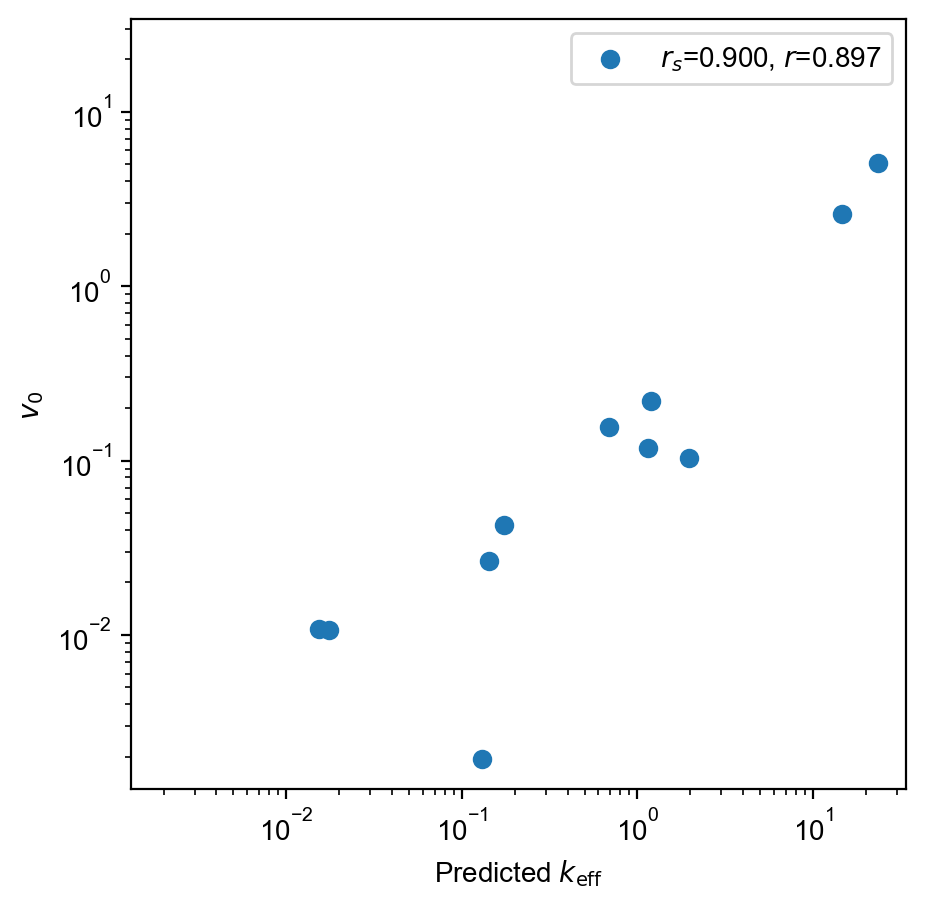
Validation

HPLC

validation_df = pyprobound.get_dataframe(["Src_HPLC.tsv"])
validation_ct = pyprobound.CountTable(validation_df, alphabet)

# Can manually score and plot sequences
observed = validation_ct.target[:, 0]
with torch.inference_mode():
    predicted = torch.exp(round_1_5m.log_aggregate(validation_ct.seqs))
spearman_r = scipy.stats.spearmanr(observed.log(), predicted.log()).statistic
pearson_r = scipy.stats.pearsonr(observed.log(), predicted.log()).statistic
plt.figure(figsize=(5, 5))
plt.scatter(
    predicted, observed, label=f"$r_s$={spearman_r:.3f}, $r$={pearson_r:.3f}"
)
plt.xscale("log")
plt.yscale("log")
plt.xlim(min(plt.xlim()[0], plt.ylim()[0]), max(plt.xlim()[1], plt.ylim()[1]))
plt.ylim(plt.xlim())
plt.xlabel(r"Predicted $k_{\mathrm{eff}}$")
plt.ylabel(r"$v_0$")
plt.legend()
plt.show()

# Or use built-in validation module with error bars
fit = pyprobound.fitting.LogFit(
    round_1_5m,
    validation_ct,
    prediction=lambda log_aggregate: log_aggregate,
    device="cpu",
    update_construct=True,
    name="Src HPLC",
)
fit.plot(
    xlabel=r"Predicted $k_{\mathrm{eff}}$",
    ylabel=r"$v_0$",
    labels=[
        "High",
        "F8-Y442",
        "F8-K444R",
        "TGM1-Y312",
        "TGM1-R315L",
        "VHL-Y185",
        "VHL-L184R",
        "HRAS-Y64",
        "HRAS-E63K",
        "CDK5-Y15",
        "CDK5-G16R",
    ],
    colors=(
        ["black"]
        + ["blue"] * 2
        + ["brown"] * 2
        + ["purple"] * 2
        + ["green"] * 2
        + ["red"] * 2
    ),
)