This example is taken from the ProBound web server, and corresponds to Figure 4 in the original Nature Biotech publication.

This example produces a single Dll binding model by training on Kd-seq data, which is an extension of a SELEX assay that sequences both the bound and unbound fractions, allowing for the calculation of absolute Kd’s from sequencing data.

import math

import pandas as pd
import torch
import scipy.stats
import matplotlib.pyplot as plt
import torch.nn.functional as F

import pyprobound
import pyprobound.plotting
import pyprobound.fitting

Data specification

alphabet = pyprobound.alphabets.DNA()

dataframe = pyprobound.get_dataframe(
    "http://pbdemo.x3dna.org/files/example_data/"
    "KD-single/countTable.0.20201205_DlldN-12.tsv.gz"
)
dataframe.head()

	1	2	3
0
AAAAAAAAAA	2	0	5
AAAAAAAAAC	3	0	3
AAAAAAAAAG	3	0	0
AAAAAAAAAT	2	0	4
AAAAAAAACA	2	0	5

count_table = pyprobound.CountTable(
    dataframe,
    alphabet,
    left_flank="GAGTTCTACAGTCCGACCTGG",
    right_flank="CCAGGACTCGGACCTGGA",
    left_flank_length=6,
    right_flank_length=6,
)

Model specification

PSAMs

nonspecific = pyprobound.layers.NonSpecific(alphabet=alphabet, name="NS")
psam = pyprobound.layers.PSAM(
    kernel_size=10,
    alphabet=alphabet,
    pairwise_distance=9,
    seed=["--TAATTG--"],
    seed_scale=6,
    name="Dll",
)

Modes

modes = [
    pyprobound.Mode.from_nonspecific(nonspecific, count_table),
    pyprobound.Mode.from_psam(psam, count_table),
]

Rounds

initial_round = pyprobound.rounds.InitialRound()
bound_round = pyprobound.rounds.BoundRound.from_binding(
    modes, initial_round, target_concentration=100, library_concentration=20
)
unbound_round = pyprobound.rounds.UnboundRound.from_round(bound_round)

Experiment

experiment = pyprobound.Experiment(
    [initial_round, bound_round, unbound_round],
    name="Dll",
    counts_per_round=count_table.counts_per_round,
)

Model

model = pyprobound.MultiExperimentLoss([experiment], pseudocount=200)

Fitting

optimizer = pyprobound.Optimizer(
    model,
    [count_table],
    greedy_threshold=2e-4,
    device="cpu",
    checkpoint="Dll.pt",
    output="Dll.txt",
)

optimizer.train_sequential()

tensor(0.9410)

optimizer.reload()

{'time': 'Wed Apr 24 02:43:16 2024',
 'version': '1.3.1',
 'flank_lengths': ((6, 6),)}

Loss

with torch.inference_mode():
    loss, reg = model([count_table])
    print(loss, reg, loss + reg)

tensor(0.8029) tensor(0.1381) tensor(0.9410)

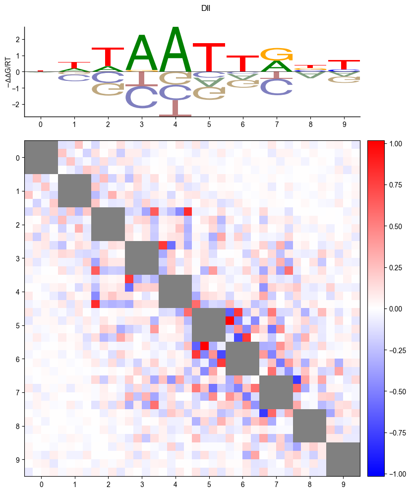
Logo

pyprobound.plotting.logo(psam)
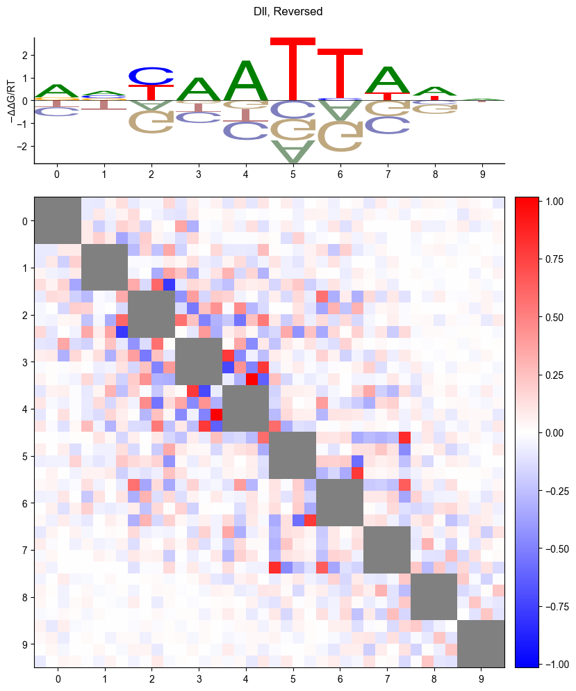
pyprobound.plotting.logo(psam, reverse=True)

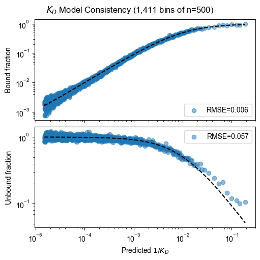
Model consistency

pyprobound.plotting.kd_consistency(experiment, 0, 1, 2, count_table)

../_images/de641ad273e1c3e47439ff550f3fc5516fcc6ce0f90201378c5d36443be625a3.png

Validation

EMSA

validation_df = pyprobound.get_dataframe(["Dll_EMSA.tsv"])
validation_ct = pyprobound.CountTable(
    validation_df,
    alphabet,
    left_flank=count_table.left_flank,
    right_flank=count_table.right_flank,
    left_flank_length=count_table.left_flank_length,
    right_flank_length=count_table.right_flank_length,
)
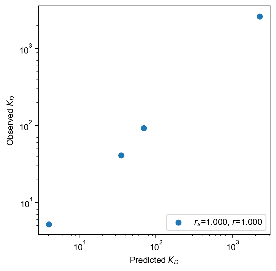
val_free_protein = experiment.free_protein(0, 1, 2, library_concentration=6.7)

# Can manually score and plot sequences
observed = validation_ct.target.squeeze()
with torch.inference_mode():
    predicted = val_free_protein / torch.exp(
        bound_round.log_aggregate(validation_ct.seqs)
    )
spearman_r = scipy.stats.spearmanr(observed.log(), predicted.log()).statistic
pearson_r = scipy.stats.pearsonr(observed.log(), predicted.log()).statistic
plt.scatter(
    predicted, observed, label=f"$r_s$={spearman_r:.3f}, $r$={pearson_r:.3f}"
)
plt.xscale("log")
plt.yscale("log")
plt.axis("scaled")
plt.xlabel(r"Predicted $K_D$")
plt.ylabel(r"Observed $K_D$")
plt.legend(loc="lower right")
plt.show()

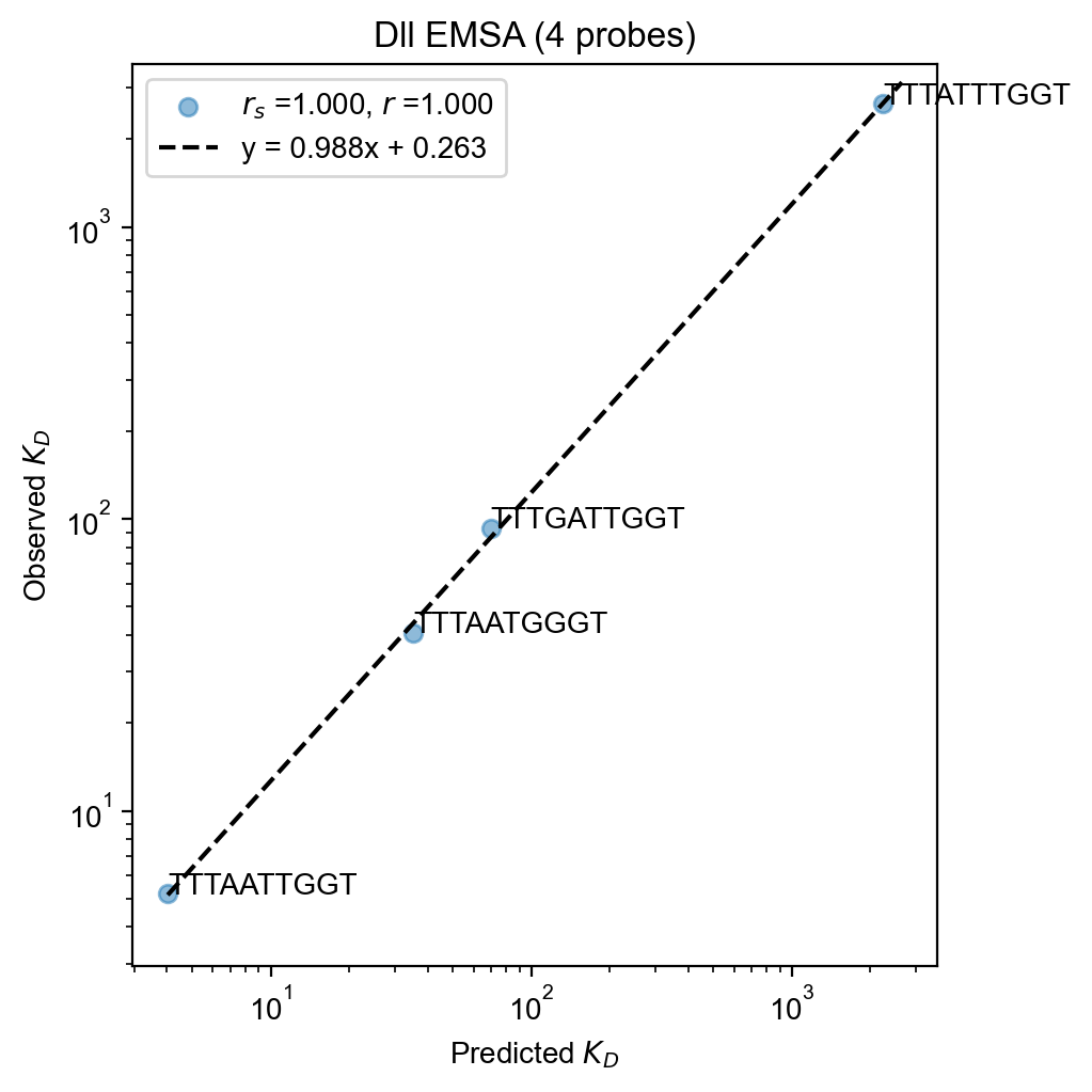
../_images/5c425eb65d1c487b1d4ac3848e3557fc797389ae479380bb675931393148358b.png

# Or use built-in validation module
prediction = lambda log_aggregate: math.log(val_free_protein) - log_aggregate
fit = pyprobound.fitting.LogFit(
    bound_round,
    validation_ct,
    prediction,
    device="cpu",
    update_construct=False,
    name="Dll EMSA",
)
fit.plot(
    labels=validation_df.index,
    xlabel=r"Predicted $K_D$",
    ylabel=r"Observed $K_D$",
)

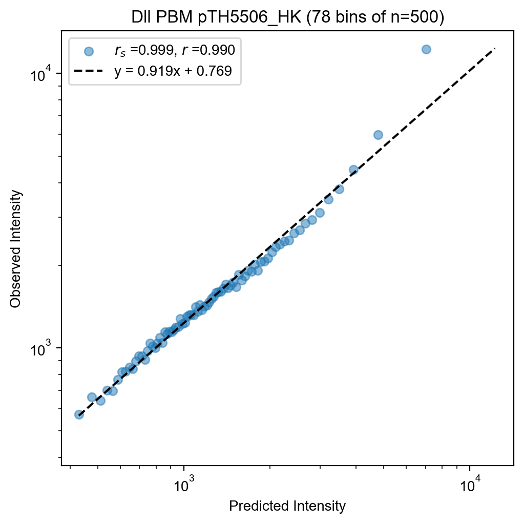
../_images/4ee117e41b8a2f5c25450bd509d240a12dd54f85a1051367b1cef67a47a3f1d6.png

PBM

# PBM table generated from Weirauch et al. (2014)
pTH5506_HK_df = pd.read_csv(
    (
        "https://www.ncbi.nlm.nih.gov/geo/download/"
        "?acc=GSM1291486&format=file&file=GSM1291486"
        r"%5FpTH5506%5FHK%5F8mer%5F2086%2Eraw%2Etxt%2Egz"
    ),
    header=0,
    index_col=None,
    sep="\t",
    compression="gzip",
)
pTH5506_HK_df.index = (
    pTH5506_HK_df["linker_sequence"] + pTH5506_HK_df["pbm_sequence"]
)
pTH5506_HK_df = pTH5506_HK_df.loc[pTH5506_HK_df["control"] == "FALSE"]
pTH5506_HK_df = (
    pTH5506_HK_df["mean_signal_intensity"]
    - pTH5506_HK_df["mean_background_intensity"]
).to_frame()
pTH5506_HK_ct = pyprobound.CountTable(
    pTH5506_HK_df, alphabet, right_flank="-" * 9, right_flank_length=9
)
pTH5506_HK_df.head()

	0
CCTGTGTGAAATTGTTATCCGCTCTGCCAGTTTAGGTGGCGCCCGGAACCCTTAACCCAT	1335.8308
CCTGTGTGAAATTGTTATCCGCTCTCATGTAGAGCCCTAAAACTGGGACTAAGCCGACCT	1369.9194
CCTGTGTGAAATTGTTATCCGCTCTGGACGCAACATGCAGCTGCACAAGTCACTTGTGAG	2527.1627
CCTGTGTGAAATTGTTATCCGCTCTAAGATTGACACGAGACTATCCAGTATACCCCTTTC	1905.6660
CCTGTGTGAAATTGTTATCCGCTCTGTGCTCGAAGAAAGGGCCACCGCGTCCCTCGCTAG	1392.8326

fit = pyprobound.fitting.LogFit(
    bound_round,
    pTH5506_HK_ct,
    prediction=F.logsigmoid,
    update_construct=True,
    train_offset=True,
    train_posbias=True,
    train_hill=True,
    device="cpu",
    name="Dll PBM pTH5506_HK",
    checkpoint="Dll_pTH5506_HK.pt",
)
fit.fit()
fit.plot(kernel=500, xlabel="Predicted Intensity", ylabel="Observed Intensity")

../_images/7d4e0dd2fb2490bd6037d6762cd350f50e2984839a88070cf01926cc7b4e7a05.png